ElaStic@exciting: How to Calculate Elastic Constants

by Rostam Golesorkhtabar, Pasquale Pavone, & Konstantin Lion for exciting oxygen

Purpose: In this tutorial you will learn how to set up and execute exciting calculations using the ElaStic@exciting interface, which allows to obtain full elastic tensors (elastic constants) of crystal systems for any crystal structure. In addition, the application of ElaStic@exciting to the determination of the elastic constants of C in the diamond phase and of hexagonal Be is explicitly presented.

---

0. Define relevant environment variables

Read the following paragraphs before starting with the rest of this tutorial!

Before starting, be sure that relevant environment variables are already defined as specified in How to set environment variables for tutorials scripts. Here is a list of the scripts which are relevant for this tutorial with a short description.

• [e-mail]: Python script for generating structures at different strains.
• [e-mail]: (Bash) shell script for running a series of exciting calculations.
• [e-mail]: Python script for fitting the energy-vs-strain and CVe-vs-strain curves.
• [e-mail]: (Bash) shell script for cleaning unnecessary files.
• [e-mail]: Python script for calculating elastic constants.
• ElaStic_Result_Energy_2nd.py: Python script for calculating second-order elastic constants.
• ElaStic_Result_Energy_3rd.py: Python script for calculating third-order elastic constants.
• ElaStic_xyz2XYZ.py: Python script for the conversion of second-order elastic constants to different coordinate systems.
• exciting2sgroup.py: Python script for converting the exciting input to an sgroup input file.
• Grace.par: File containing xmgrace parameters needed by visualization tools.

Requirements: Bash shell. Python numpy, lxml, math, sys and os libraries. xmgrace (visualization tool).

From now on the symbol $ will indicate the shell prompt.

Extra requirement: Tool for space-group determination

The scripts in this tutorial use the sgroup tool. If you have not done before, this tool should be downloaded and installed.

---

☛ How to check if sgroup is already installed

In order to check if sgroup is already installed in the computer you are working, write on the command line:

$ sgroup

Two possible messages may appear now on the screen.

• First case: sgroup is already installed:

No input file specified.

• Second case: sgroup must be installed:

bash: sgroup: command not found

---

☛ How to install sgroup

The code sgroup is a utility which allows to determine the space group and symmetry operations of a crystal structure.

• Tool name: sgroup
• Authors: B.Z. Yanchitsky, A.N. Timoshevskii
• Download sgroup here

After the download, you will get the adon_v1_0.tar.gz file, go to the directory where you saved this file and execute the following commands.

$ tar xfvp adon_v1_0.tar.gz
$ cd SpaceGroups
$ make
$ cp sgroup $EXCITINGTOOLS

Now, you have everything you need for starting and performing general lattice optimization.

---

1. Set up the calculations

i) Preparation of the input file

The first step is to create a directory for each system that you want to investigate. In this tutorial, we first consider as an example carbon in the diamond structure (the procedure we use is, nevertheless, valid for any system). Thus, we will create a directory C_2nd and we move inside it.

$ mkdir C_2nd
$ cd C_2nd

Inside this directory, we create or copy an optimized structure file for diamond named input.xml. This file could look like the following.

<input>
 
   <title>Diamond: 2nd-order elastic constants</title>
 
   <structure speciespath="$EXCITINGROOT/species">
 
      <crystal scale="6.7165">
         <basevect> 0.5  0.5  0.0 </basevect>
         <basevect> 0.5  0.0  0.5 </basevect>
         <basevect> 0.0  0.5  0.5 </basevect>
      </crystal>
 
      <species speciesfile="C.xml" rmt="1.30">
         <atom coord="0.00  0.00  0.00"/>
         <atom coord="0.25  0.25  0.25"/>
      </species>
 
   </structure>
 
   <groundstate 
      xctype="GGA_PBE_SOL"
      ngridk="6 6 6"
      swidth="0.0001"
      gmaxvr="18"
      maxscl="30">
   </groundstate>
 
   <relax/>
 
</input>

To the purposes of this tutorial, this file can be saved with any name. However, notice that the input file for a direct exciting calculation must be always called input.xml.

Be sure to set the correct path for the exciting root directory (indicated in this example by $EXCITINGROOT) to the one pointing to the place where the exciting directory is placed. In order to do this, use the command

$ SETUP-excitingroot.sh

ii) Generation of input files for distorted structures

All strains considered in this tutorial are Lagrangian strains.

In order to generate input files for a series of distorted structures, you have to run the script [e-mail], which will produce the following output on the screen.

$ [e-mail]

     2nd  ---=>  2           
     3rd  ---=>  3    
>>>> Please choose the order of the elastic constant (choose '2' or '3'): 2

>>>> Please enter the exciting input file name: input.xml         

     Number and name of space group: 227 (F d -3 m) [origin choice 2]       
     Cubic I structure in the Laue classification.       
     This structure has 3 independent second-order elastic constants.

>>>> Please enter the maximum Lagrangian strain 
     The suggested value is between 0.030 and 0.150: 0.05
     The maximum Lagrangian strain is 0.05

>>>> Please enter the number of the distorted structures [odd number > 4]: 11
     The number of the distorted structures is 11

$

Entry values must be typed on the screen when requested. In this case, the entries are the following.

1. 2, the order of the elastic constants in which you are interested.
2. input.xml, the name of the input file.
3. 0.05, the absolute value of the maximum strain for which we want to perform the calculation.
4. 11, the number of deformed structures equally spaced in strain, which are generated between the maximum negative strain and the maximum positive one.

The script generates some new directories and files, which you can list using the following command (in the C_2nd directory).

$ ls
input.xml  Distorted_Parameters  Dst01  Dst02  Dst03  INFO_ElaStic  Structures_exciting  sgroup.out
$

You may also list the single directories, e.g., if you list Dst01 you will see the following (sub)directories.

$ ls Dst01
Dst01_01  Dst01_02  Dst01_03  Dst01_04  Dst01_05  Dst01_06  Dst01_07  Dst01_08  Dst01_09  Dst01_10  Dst01_11
$

---

3. Execute the calculations

To execute the series of calculations, run (in the C_2nd directory) the script [e-mail], which will produce an output on the screen similar to the following.

$ [e-mail] 

        +--------------------------------------+
        | SCF calculation of "Dst01_01" starts |
        +--------------------------------------+
   Elapsed time = 0m8s

        +--------------------------------------+
        | SCF calculation of "Dst01_02" starts |
        +--------------------------------------+
   Elapsed time = 0m8s

        +--------------------------------------+
        | SCF calculation of "Dst01_03" starts |
        +--------------------------------------+

...

        +--------------------------------------+
        | SCF calculation of "Dst03_11" starts |
        +--------------------------------------+
   Elapsed time = 0m40s
$

After the complete run, elastic constants can be calculated.

The running time necessary for performing a complete calculation of the elastic constants of diamond using computational parameters as included in the above file input.xml, is less than one hour (depending on the machine processor you are using).

---

4. Analyzing the calculations

Elastic constants are obtained from energy calculations using a similar method to the one illustrated in Energy vs. strain calculations. Within this approach, second derivatives of the energy curves are evaluated with the help of a curve fitting. Calculations performed above were producing 11 points for each energy curve.

Now, in order to calculate elastic constants, we have to analyze our calculations. The script [e-mail] allows the analysis of the dependence of the calculated derivatives of the energy-vs-strain curve on

1. the range of distortions included in the fitting procedure (the x axis in xmgrace plots),
2. the degree of the polynomial fit used in the fitting procedure (different color curves in xmgrace plots).

The [e-mail] script is executed as follows.

$ [e-mail]

At this point, three xmgrace plots will appear on your screen automatically (for more information on how to deal with xmgrace plots, see Xmgrace: A Quickstart). The plots should be similar to the ones displayed in the following.

• Results for the distortion Dst01

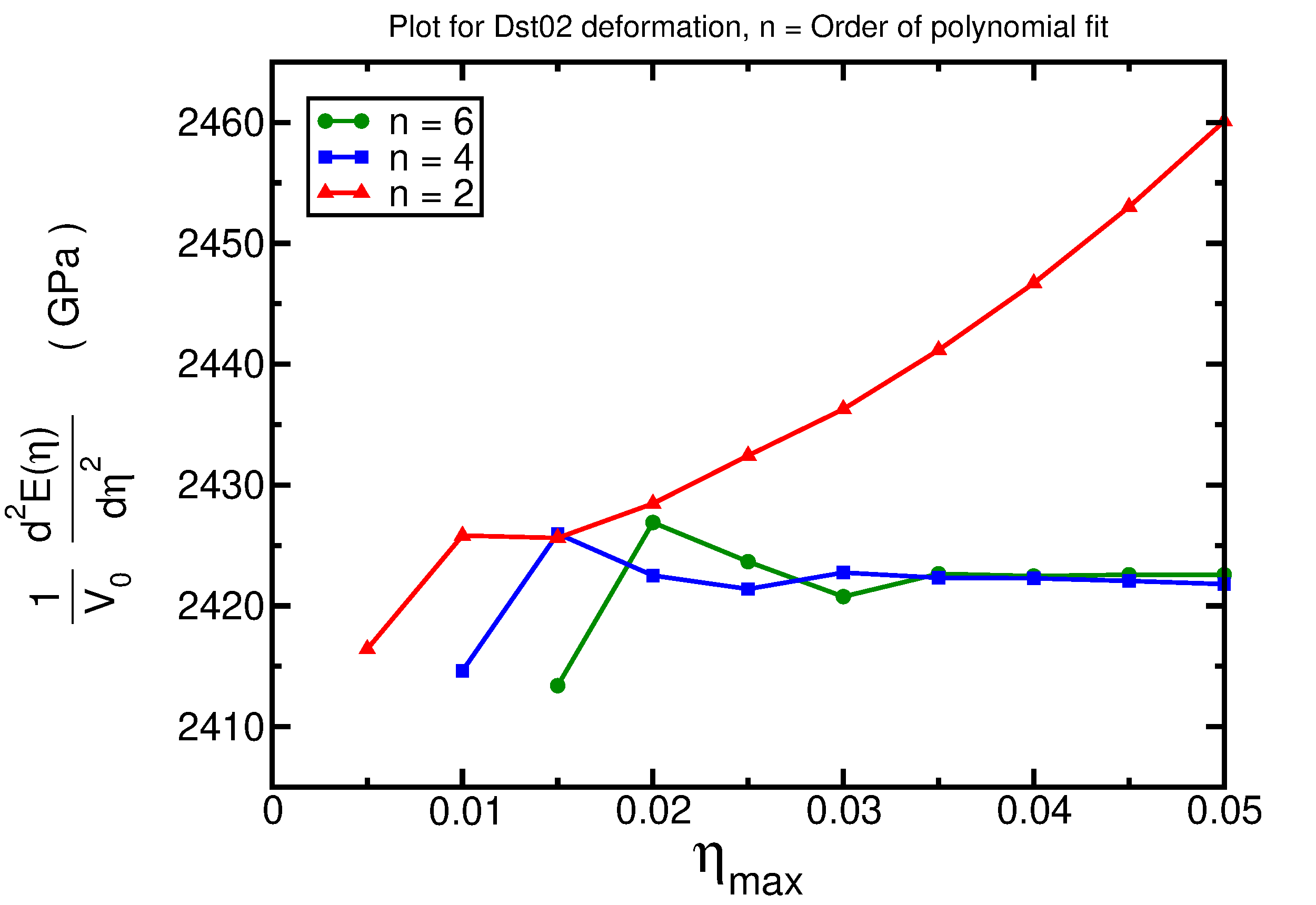
• Results for the distortion Dst02

• Results for the distortion Dst03

The previous plots can be used to determine the best range of deformations and order of polynomial fit for each distortion.

As an example, we analyze the first plot, corresponding to the distortion Dst01. Distortion types are listed in the file Distorted_Parameter. By examining this file, we can see that the Dst01 distortion corresponds to an applied Lagrangian strain in the Voigt notation with the form (η,η,η,0,0,0), where η is a strain parameter. This deformation type is directly connected with the bulk module B₀. For each distortion type, a plot appears. This plot contains the second derivative of the energy with respect to the strain parameter η as a function of the maximum strain and of the order of polynomial fit. By analyzing the plot for the Dst01 distortion, we notice that curves corresponding to the higher order of the polynomial used in the fit show a horizontal plateau at about 4040-4045 GPa. This can be assumed to be the optimal value for the second derivative, from the point of view of the fit and corresponding to the choice of the other computational parameters (further information on this topic can be found here). For this distortion type, this value equals 9 times the bulk modulus. Thus, the extracted value of the bulk modulus is about 449 GPa.

As we have mentioned before many times, the quality of the results strongly depends on the numerical parameters used for the calculation. A better converged result (using a 10$\times$10$\times$10 k-grid, rgkmax = "8.0", and 21 deformed structures) can be found below.

---

☛ show converged plots

Hint: Run converged calculation in a different directory, e.g., /home/tutorial/C_2nd-conv.

$ mkdir /home/tutorial/C_2nd-conv
$ cd /home/tutorial/C_2nd-conv

Copy here the previous input.xml and modify the computational parameters. Be aware that the run times of these computations are significantly larger than the previous ones. The result should look like the following.

• Results for the distortion Dst01

• Results for the distortion Dst02

• Results for the distortion Dst03

---

5. Numerical values of the elastic constants

The script [e-mail] used in the previous section, generates the file ElaStic_2nd.in, which will be discussed here. In order to obtain the numerical values of the second-order elastic constants of diamond, you should use the following procedure. The first step is to edit the file ElaStic_2nd.in, which should have the form

Dst01     eta_max     Fit_order
Dst02     eta_max     Fit_order
Dst03     eta_max     Fit_order

In each row of this file, you should insert a value for eta_max and Fit_order. According to the result of the visual analisys of the previous figures, these two values are extracted by considering the plateau regions of the corresponding plot: eta_max is a value of maximum distortion located in the plateau region of the curve representing the polynomial fit of order Fit_order. In our case, we can choose the parameters as listed in the example ElaStic_2nd.in below

Dst01     0.05     6
Dst02     0.05     6
Dst03     0.05     6

Now, in order to calculate elastic constants and moduli, you should run the [e-mail] script.

$ [e-mail]

Finally, numerical values of the elastic constants for diamond are written in the output file ElaStic_2nd.out.

Experimental reference elastic constants for diamond:

• C₁₁ = 1076 GPa
• C₁₂ = 125 GPa
• C₄₄ = 577 GPa
• B₀ = 452 GPa

---

6. Set up the calculation for Be

In the next example, we consider the calculation of the elastic constants of hexagonal Be.

First, create a new directory Be_2nd and move inside it.

$ mkdir Be_2nd
$ cd Be_2nd

Inside this directory, create the file input.xml corresponding to the optimized input file for the equilibrium structure of Be.

<input>
 
   <title>Be: 2nd-order elastic constants</title>
 
   <structure speciespath="$EXCITINGROOT/species">
 
      <crystal scale="4.3207">
         <basevect>  1.00000000  0.00000000  0.00000000 </basevect>
         <basevect> -0.50000000  0.86602540  0.00000000 </basevect>
         <basevect>  0.00000000  0.00000000  1.52257736 </basevect>
      </crystal>
 
      <species speciesfile="Be.xml" rmt="1.85">
         <atom coord="0.66666667  0.33333333  0.75000000"/>
         <atom coord="0.33333333  0.66666667  0.25000000"/>
      </species>
 
   </structure>
 
   <groundstate 
      xctype="GGA_PBE_SOL"
      ngridk="6 6 4"
      rgkmax="6.5"
      maxscl="30">
   </groundstate>
 
   <relax/>
 
</input>

Do not forget to update the string "$EXCITINGROOT" inside the file input.xml.

Then, we generate a set of exciting input files with the script [e-mail].

$ [e-mail]

     2nd  ---=>  2           
     3rd  ---=>  3    
>>>> Please choose the order of the elastic constant (choose '2' or '3'): 2

>>>> Please enter the exciting input file name: input.xml         

     Number and name of space group: 194 (P 63/m m c)       
     Hexagonal I structure in the Laue classification.
     This structure has 5 independent second-order elastic constants.

>>>> Please enter the maximum Lagrangian strain 
     The suggested value is between 0.030 and 0.150: 0.05
     The maximum Lagrangian strain is 0.05

>>>> Please enter the number of the distorted structures [odd number > 4]: 21
     The number of the distorted structures is 21

$

From now on, the procedure is completely equivalent to the one used for diamond. The analysis of the result can be made as in the previous example. Please, notice that the numerical parameters used in this example do not guarantee full convergence of results.