How to Visualize Phonons

by Stefan Kontur for exciting fluorine

Purpose: This tutorial shows you how to visualize the phonon modes found in an earlier phonon calculation, using a basic python script. As in other tutorials, we consider the diamond crystal as example.

---

0. Prerequisites

This tutorial assumes that you have already downloaded and installed exciting, and set the relevant environment variables. Otherwise, please have a look at How to set environment variables for tutorials scripts. The script which is relevant for this tutorial is

• PLOT-phonon-anim.py

Note: The symbol $ at beginnings of lines in code segments below indicates the shell prompt.

Continue in the working directory where you did the phonon calculation, e.g., /home/tutorials/diamond-phonons/c-test. In particluar you need to have the files input.xml and PHONON.OUT ready. The script will also read the relevant species files, C.xml in our example for diamond, in the path specified by $EXCITINGROOT/species.

---

1. Produce coordinate files of the animated phonon modes

In order to create coordinate files for a given phonon, you should invoke the script PLOT-phonon-anim.py. This script will read phonon eigenvectors for all q-points contained in the file PHONON.OUT and plot a supercell of (default) 6$\times$6$\times$6 unit cells to visualize them. Unit cells are taken as specified in input.xml and the dimensions are along lattice vectors. If you want to change the supercell size, e.g., type

$ PLOT-phonon-anim.py 4 4 1

to obtain a supercell of 4$\times$4$\times$1 unit cells.

---

☛ Further options for PLOT-phonon-anim.py

If only one argument is specified, the value you give will act as a scaling factor for the atom displacements, e.g.

$ PLOT-phonon-anim.py 10.0

A scaling factor of 10.0 is the default value. For heavy atoms you might need a larger value to visualize the vibration properly. Of course, you can also specifiy both, the supercell size and a scaling factor, in this order, e.g.

$ PLOT-phonon-anim.py 6 6 6 10.0

---

When executing the script PLOT-phonon-anim.py, you will be required to enter the number of steps in the animation which complete one period of the vibration.

$ PLOT-phonon-anim.py
############################################

Supercell dimensions :      6     6     6

Number of steps in the animation? >>>> 20

--------------------------------------------
Total number of atoms    :     2
Total number of q-points :     3
--------------------------------------------

q-point  1  is  0.0 0.0 0.0
   mode  1  with frequency    -0.0000  cm-1
   mode  2  with frequency    -0.0000  cm-1
   mode  3  with frequency    -0.0000  cm-1
   mode  4  with frequency  1580.5233  cm-1
   mode  5  with frequency  1580.5233  cm-1
   mode  6  with frequency  1580.5233  cm-1

q-point  2  is  0.5 0.5 0.0
   mode  1  with frequency   523.8800  cm-1
   mode  2  with frequency   523.8800  cm-1
   mode  3  with frequency  1096.3667  cm-1
   mode  4  with frequency  1096.3667  cm-1
   mode  5  with frequency  1128.0147  cm-1
   mode  6  with frequency  1128.0147  cm-1

q-point  3  is  0.5 0.5 0.5
   mode  1  with frequency   459.4412  cm-1
   mode  2  with frequency   459.4412  cm-1
   mode  3  with frequency   869.1994  cm-1
   mode  4  with frequency  1238.7323  cm-1
   mode  5  with frequency  1400.8203  cm-1
   mode  6  with frequency  1400.8203  cm-1

############################################

$

Specify, e.g., 20 steps, as above. The screen output of the script is completed by information about the number of atoms, number of q-points, and the frequency (in cm^-1) for each mode at each q-point.

Beyond this information, the script produces a number of files, named, e.g., q1_mode1.axsf and q1_mode1.xyz. One file is written for each mode at each q-point. These files contain atomic coordinates for the supercell at every step of the animation. The files with extension axsf are animated XCrySDen structure files, the files with extension xyz are simple xyz-coordinate files.

The next subsections deal with visualizing these files. To exemplify, we show this using VMD. You might have other/additional choices, according to the actual software installed in your environment.

---

2. Visualize coordinate files

2.1) Using VMD

We make use of VMD, and assume that you have an installed and properly set up version available on you system.

After starting the program by typing

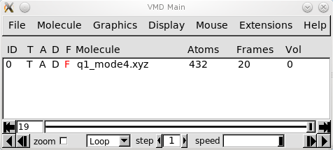
$ vmd >/dev/null 2>&1 &

Now, use the buttons File -> New Molecule to open a dialog to open files. Use Browse to choose a file in your working directory, e.g., q1_mode4.xyz, the file type should be determined automatically, and Load to yield the following windows:

Use the Graphics -> Representations button to change the appearance of atoms and bonds. In the example below the choice for Drawing Method was CPK. Colors of atoms and the background can be changed via Graphics -> Colors. You might also want to change to a non-perspective display or omit the axes in the image, using the Display menu. The animation of the phonon mode can be started and stopped using the "play" (right-pointing black triangle) button in the bottom-right corner of the VDM Main window.

Our phonon mode, the 4th one at the Γ point, would look then like the following:

As another example, let us have a look at the first acoustic mode at q = (0.1, 0.1, 0), on the line Δ (i.e., Γ-X). You have to rerun the phonon calculation with this q-point added to the list as discussed in Section 1.4 of Phonon Properties of Diamond-Structure Crystals, and invoke the script PLOT-phonon-anim.py once more, to obtain the appropriate .xyz file.

For a detailed description of all features of VMD and tutorials, including the creation of movies, we refer to the VMD website.